By Tobias Ortmayr and
Tanja Mayerhofer
Introduction
This tutorial demonstrates how to use xMOF in GEMOC Studio for developing executable domain-specific modeling languages (xDSMLs) and executing models.
For this, it will show you how to make the predefined FSM language, a simple Ecore-based language for defining finite state machines, executable with xMOF, and how to execute and debug FSM models.
To achieve this, you will learn how to perform the following steps:
- Setup GEMOC Studio with xMOF
- Import the (not yet executable) FSM language
- Create an xMOF project for the FSM language
- Define the execution semantics of the FSM language with xMOF
- Generate code for the FSM xMOF model
- Create an xDSML project for the FSM language
- Create an animator project for the FSM language
- Launch the modeling workbench for the FSM language
- Execute an FSM model
The complete FSM example is also provided together with the xMOF component of GEMOC Studio.
In the end of the tutorial, you find instructions on
how to install the example.
1. Setup GEMOC Studio with xMOF
For setting up GEMOC Studio, download the latest version of GEMOC Studio from
gemoc.org.
The download will deliver a compressed
zip or
tar.gz archive.
Decompress this archive into a directory of your choice and ensure you have full read and execute permissions for this directory.
Start GEMOC Studio by running
GemocStudio.exe on Windows or
GemocStudio on other platforms.
xMOF is provided as an additional component of GEMOC Studio.
To install it, open the menu
Help and select
Install Additional GEMOC Components. Select from the category
Alternative GEMOC based Engines the component
GEMOC xMOF Engine.
After selecting the component
GEMOC xMOF Engine, hit the
Finish button.
Confirm the
Install and
Install Details dialogs by hitting
Next, read and accept the license agreement and hit
Finish.
Confirm the warning about installing unsigned content and restart GEMOC Studio.
2. Import the FSM Language
The FSM language is a simple language for defining finite state machines.
Its abstract syntax is defined by an Ecore model.
For graphically visualizing FSM models, a Sirius-based editor is also provided for the language.
We will see in this section how we can import the EMF projects implementing the FSM language and have a look inside these projects.
Download the FSM Implementation Projects
The EMF projects implementing the FSM language can be downloaded as an archive file
fsa-tutorial.zip from
modelexecution.org.
Import the FSM Implementation Projects
For importing the downloaded projects, open the menu
File and select
Import...
In the opening
Import wizard, select
General /
Existing Projects into Workspace.
Chose the downloaded archive file
fsa-tutorial.zip under the option
Select archive file and select all projects located in the directory
language_workbench.
Abstract Syntax
FSM models are simple I/O state machines.
The abstract syntax of the FSM language is defined by the Ecore model
fsm.ecore located in the imported project
org.modelexecution.xmof.examples.fsm.
As you can see from the Ecore model, a
finite state machine (FSM) is a set as of
states and
transitions.
One state serves as
initial state.
Each transition has exactly one
source state and exactly one
target state.
In addition, each transition defines an
input String and an
output String.
For each state, the inputs of outgoing transitions must be distinct to avoid non-deterministic state machines.
Concrete Syntax
The graphical concrete syntax for visualizing FSM models is defined by the Sirius viewpoint specification model
fsm.odesign contained by the imported project
org.modelexecution.xmof.examples.fsm.design.
It depicts states as circles and transitions as edges with their
input /
output Strings as label.
The example shows a simple finite state machine that accepts the input String “HELLO!” and produces the output String “WORLD!”.
3. Create an xMOF Project
To make the FSM language executable, we have to first create a new xMOF project for the FSM language.
To create a new xMOF project, open the menu
File and select
New >
Other....
Select in the category
xMOF the entry
xMOF Project.
In the appearing dialog
New xMOF Project, you have to provide the name of the xMOF project and the name of the executable language that is going to be developed.
For the FSM example, we chose the following names:
- Project name: org.modelexecution.xmof.examples.fsm.xmof.dynamic
- Language name: FSM
Confirm the input by hitting the
Next button.
On the next page
Ecore Metamodel File, you have to select the Ecore model defining the abstract syntax of your language.
For this, click on
Browse Workspace, unfold the project
org.modelexecution.xmof.examples.fsm, select the file
fsm.ecore and hit
OK.
The content of the Ecore model will then be displayed in the wizard page.
As last step you have to select the main class of your Ecore model.
This class will serve as entry point for the execution of FSM models.
Select the class
FSM as main class and hit
Finish.
The wizard created for you the new xMOF project
org.modelexecution.xmof.examples.fsm.xmof.dynamic containing a new xMOF model
fsm.xmof.
This xMOF model provides configuration classes for all classes of the FSM Ecore model and will be used in the next step for defining the execution semantics of our FSM language.
4. Define the Execution Semantics of FSM with xMOF
In this step, we will define the execution semantics of the FSM language.
This is done in the created xMOF model
fsm.xmof.
We will have to define the following components common to the execution semantics of xDSMLs:
- Dynamic elements defining the runtime states of models
- Input parameters accepted for the execution of models
- Behavior of the model elements
Before we go into the details on how to define these elements for FSM, we will first have a look at the desired execution behavior of FSM models.
Desired Execution Behavior
When executing an FSM model we want to process a sequence of input Strings and determine the output String produced by the finite state machine.
For doing that, it is checked for each String in the input sequence whether one of the outgoing transitions of the currently active state can process it.
A transition can process a String when it is equal to the
input String defined by the transition.
A finite state machine starts with the
initial state as first active state.
If a transition can process the current input String, the transition is fired.
When a transition is fired, the transition
output String is added to the output String starting with an empty String, and the target state of the transition is set as the new active state.
4.1. Define Dynamic Elements
To achieve the desired execution behavior we need a way to define the currently active state of a finite state machine as well as the output String of a state machine.
In addition, we also need to store information about the accepted input sequence of Strings.
This is referred to as the
runtime state of a finite state machine.
To define the runtime state of an FSM model, we therefore extend the configuration class
FSMLConfiguration with a reference
currentState to the
State class, and the multi-valued String attributes
producedSeq and
acceptedSeq.
4.2. Define Input Parameters
Input Elements
The input processed by a finite state machine is an arbitrary sequence of input Strings.
To enable the user of the FSM language to define such an input String sequence, we introduce the class
Input into the xMOF model owning the multi-valued String attribute
inputSeq.
Note that the property
unique of this attribute has to be set to
false to allow duplicate elements in the sequence.
Input Parameters
Finally, we have to define that an input String sequence, i.e., an instance of the newly defined class
Input, has to be provided for executing an FSML model.
To do that, we have to add an input parameter to the
main operation that was automatically added to the main class of our FSM language
FSMConfiguration.
To add this input parameter right-click on the operation
main and select
New Child >
DirectedParameter.
Change the name of the input parameter to
input and set its type to
Input.
4.3. Define Behavior
To define the above described execution behavior of finite state machines, we have to define four operations and their behavior:
- The main operation of the configuration class FSMConfiguration serving as entry point of the execution.
- The run operation of the configuration class FSMConfiguration defining the behavior of finite state machines.
- The process operation of the configuration class StateConfiguration defining the behavior of a state when processing an input String.
- The fire operation of the configuration class TransitionConfiguration defining the behavior of a transition when firing.
Add Operations
To add a new operation, right-click on the respective configuration class and select
New Child >
BehavioredEOperation.
Set the name accordingly and add appropriate parameters.
Create Activities
With xMOF, the behavior of operations is defined with UML activities.
To create the activity defining the behavior of an operation, simply double-click on the operation.
The activity will be created and initialized with parameters corresponding to the parameters defined for the respective operation.
For instance, by double-clicking on the
main operation, an activity named
main_FSMConfiguration is created.
Define Behavior of Activities
Now we can define the behavior of the created activities.
Double-clicking on an activity or operation will initialize and open the corresponding activity diagram.
We will start with the
main operation.
The palette on the right provides tools for the creation of activity nodes and activity edges.
xMOF is based on the UML action language.
Detailed descriptions of action types and other UML node types can be found in the
UML specification.
The modeling of the
main activity is covered in detail in this tutorial.
For the other activities only the final activity diagrams are shown.
Information on
how to install the complete example are given in the end of the tutorial.
main Activity
The
main activity has to first set the initial state of the finite state machine as currently active state and then to process the provided input by calling the operation
run.
Finally, it has to provide the output sequence produced by the
run operation as output of the finite state machine.
For doing this, we first need to add a
Read Self Action named
read fsm to the activity.
This action will retrieve the executing
FSM element.
Select the
Read Self Action element in the tool palette and click on the diagram.
In the appearing dialog, enter the name
read fsm and click
OK.
In the same fashion, we create the remaining needed actions.
To access the initial state of an FSM, we define a
Read Structural Feature Action called
read initialState and set its property
Structural feature to
initialState.
To set the retrieved state as currently active state, we furthermore create an
Add Structural Feature Value Action named
set currentState and set its property
Structural feature to
currentState.
To call the operation
run, we define a
Call Operation Action named
call run and set its property
Operation to
run.
Furthermore, to pass the executing FSM element on to these actions, we create a
Fork Node.
Use the properties view to set the properties
Structural feature and
Operation.
Now we can connect the created activity nodes with object flows and control flows.
To add a new flow, select the required flow type in the tool palette and then click on the nodes you want to connect.
To pass along the executing FSM element, we need to connect the output of the
read fsm action with the created fork node and the fork node with the
target and
object inputs of the actions
call run,
read initialState, and
set currentState.
Furthermore, the initial state retrieved by the
read initialState action has to be provided to the
value input of the
set currentState action.
Finally, the provided
input parameter value has to be passed on to the
run operation.
All of these flows are object flows.
However, these object flows cannot ensure that the
run operation is invoked only after the currently active state has been set to the initial state of the finite state machine.
Thus, we also need to define an additional control flow from the
set currentState action to the
call run action.
The final
main activity looks as follows:
run Activity
The
run activity reads the input String sequence provided by the input parameter value and then processes each element in the input String sequence by calling the
process operation of the current state.
The iteration over the input String sequence can be defined with an
Expansion Region.
The activity nodes contained by the expansion region are executed for each element of the provided input String sequence.
process Activity
The
process activity determines for the current state whether one of its outgoing transitions can process the currently processed input String, i.e., whether one of its outgoing transitions defined the String as processable
input.
If such a transition is found, this transition is fired by calling its
fire operation.
Note that for the outgoing control flow of the decision node, a guard has to be defined.
This has to be done in the tree editor.
Switch to the tree editor by clicking on the
Selection tab shown in the bottom left corner of the editor.
Right-click on the object flow and select
New Child >
Guard Literal Boolean.
Then set its
Value property to
true using the properties view.
fire Activity
The
fire activity of a transition has to perform the following tasks:
It has to set the target state of the transition as the new current state of the FSM, add the output of the transition to the produced String sequence, and add the processed input String to the accepted String sequence.
5. Generate Code for an xMOF Model
After the xMOF model has been completely defined, we have to generate Java code for it.
To do this, right-click in the project explorer on the xMOF project
org.modelexecution.xmof.examples.fsm.xmof.dynamic and select
xMOF >
Generate Code.
The Java code is generated in the
src foder of the xMOF project.
Please note that the Java code has to be re-generated whenever the xMOF model is updated.
6. Create an xDSML Project
As a next step, we have to create a GEMOC xDSML project for the FSM language that identifies the FSM language as executable language.
The GEMOC xDSML project can be automatically generated for an xMOF project.
For this, right-click in the project explorer on the xMOF project
org.modelexecution.xmof.examples.fsm.xmof.dynamic and select
xMOF >
Generate xDSML Project.
The generation of the Java code an the xDSML project can be also achieved in one step by right-clicking in the project explorer on the xMOF project
org.modelexecution.xmof.examples.fsm.xmof.dynamic and selecting
xMOF >
Generate All.
7. Create an Animator Project
After completing the previous steps, you can already execute FSM models.
If you are not interested in animating executing FSM models, you can skip this step and proceed with
Step 9.
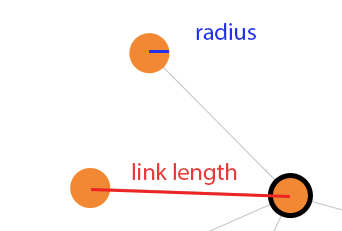
Desired Animation
During the execution of an FSM model, we want to visualize:
- The currently active state in red color
- The String sequence that the FSM has accepted so far
- The String sequence that the FSM has produced so far
Add Animation Layer
To implement the desired animation, we first need to add an animation layer and corresponding animation service classes to the Sirius viewpoint specification model.
For this, open the Sirius viewpoint specification model of the FSM language
fsm.odesign located in the project
org.modelexecution.xmof.examples.fsm.design.
Right-click on the
FSMDiagram element and select
xMOF >
Add Animation Layer.
This adds a dedicated layer called
Animation to the diagram and initializes the
FsmdiagramAnimationServices class.
Extend Animation Service Class
To display the produced and accepted String sequences we need simple methods that concatenate all elements of the sequence to one single String.
In addition, the order needs to be reversed as the elements are added in last-in/first-out order during execution.
For this, we extend the class
FsmdiagramAnimationServices with two simple service methods as shown below:
Note that after adding the methods you may get some import errors which can be easily resolved with the Eclipse Quickfix feature.
Extend Animation Layer to Highlight the Current State
To display the currently active state in red color, we can use a style customization.
In the Sirius specification editor navigate to the
Animation layer.
Then right-click on
Style customizations and select
New Customization >
Style Customization.
As predicate expression for this customization define
[self.containingFSM.oclAsType(fsmConfiguration::FSMConfiguration).currentState=self/].
Then right-click on the the style customization and select
New Customization >
Property Customization (by selection) and set the
property values as shown below:
Extend Animation Layer to Display Information on the Accepted and Produced String Sequences
To display the accepted and produced Strings, we create a container mapping called
ExecutionInfo in the
Animation layer and contained node mappings called
AcceptedString and
ProducedString as shown below.
For these mappings set the property
Domain Class to
fsm.Fsm and the
Semantic Candidate Expression to
[self/].
In addition, change the property
Child Representation of
ExecutionInfo to
list.
For the label expressions of the basic shapes of
AcceptedString and
ProducedString use the following values:
- ['Accepted String: '+self.getAcceptedString()/]
- ['Produced String: '+self.getProducedString()/]
8. Launch the Modeling Workbench
Now we have completely implemented the executable FSM language and a corresponding animator, and are ready to execute and debug FSM models.
For this, we start the FSM modeling workbench.
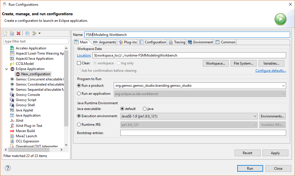
Expand the
Run control in the menu bar and select
Run Configurations....
Double-click on
Eclipse Application, change the name to
FSM Modeling Workbench, and click on
Run to start the FSM modeling workbench.
Import the project
org.modelexecution.xmof.examples.fsm.samplemodels from the folder
modeling_workbench of the downloaded archive file
fsm-tutorial.zip into the modeling workbench.
For this, open the menu
File, select
Import... >
General /
Existing Projects into Workspace, browse to the archive file, select the sample model project, and hit
Finish.
The imported project contains the introduced
Hello World example and another example defining a finite state machine for traffic lights.
To open an example model make sure that you are in the
Modeling perspective.
The perspective can be changed with the menu
Window >
Open Perspective >
Others.
Open the Hello World example by double-clicking on the
HelloWorld.aird file.
Then, expand the aird file until the
FSMDiagram appears.
Open it by double-clicking.
9. Execute an FSM Model
To execute the Hello World finite state machine, expand the
Debug control in the menu bar and select
Debug Configurations...
Double-click on
xMOF Executable Model.
Change the name of the new configuration to
HelloWorld.
Select
HelloWorld.fsm as the model to execute and
HelloWorld.parameters1.xmi as the initialization model.
Select the melange language
org.modelexecution.xmof.examples.fsm.Fsm and the animator
HelloWorld.aird.
Finally, click on
Debug.
The Hello World FSM model now starts executing.
After the execution engine has been started, a dialog
Confirm Perspective Switch will appear.
Click on
Yes and the debugging perspective will be opened.
Interact with the debugging model using the usual Eclipse debug commands.
Use the control
Step Into from the menu bar to execute the Hello World model step-by-step.
The model will be animated showing the currently active state, the processed input Strings and the produced output Strings.
The
stack trace view shows the next execution step to be performed and the
variables view shows the current values of the different model elements.
Below you can see the animation of the model after stepping three times.
Congratulations! You have defined your first xDSML with xMOF.
Getting the Complete Example
The complete FSM example is delivered with the xMOF component of GEMOC Studio.
To install it open the
File menu, select
New >
Other... >
Examples /
xMOF Language Examples /
xMOF FSM Language, and hit
Finish.
All projects implementing the FSM language will be imported in your language workbench.
In the same way you can also import the sample model project.
Open the
File menu, select
New >
Other... >
Examples /
xMOF Modeling Examples /
Model Example for xMOF FSM Language, and hit
Finish.